Introduction

In this article I would like to discuss some nuances about the `DBSCAN` clustering algorithm. This is by no means a detailed explanation of the algorithm. The intent of this article is to demonstrate how to calculate the value of `epsilon` parameter when the various dimensions of the features follow different measurement systems. E.g., Age on X axis and Height on Y axis.

An overview of the DBSCAN algorithm

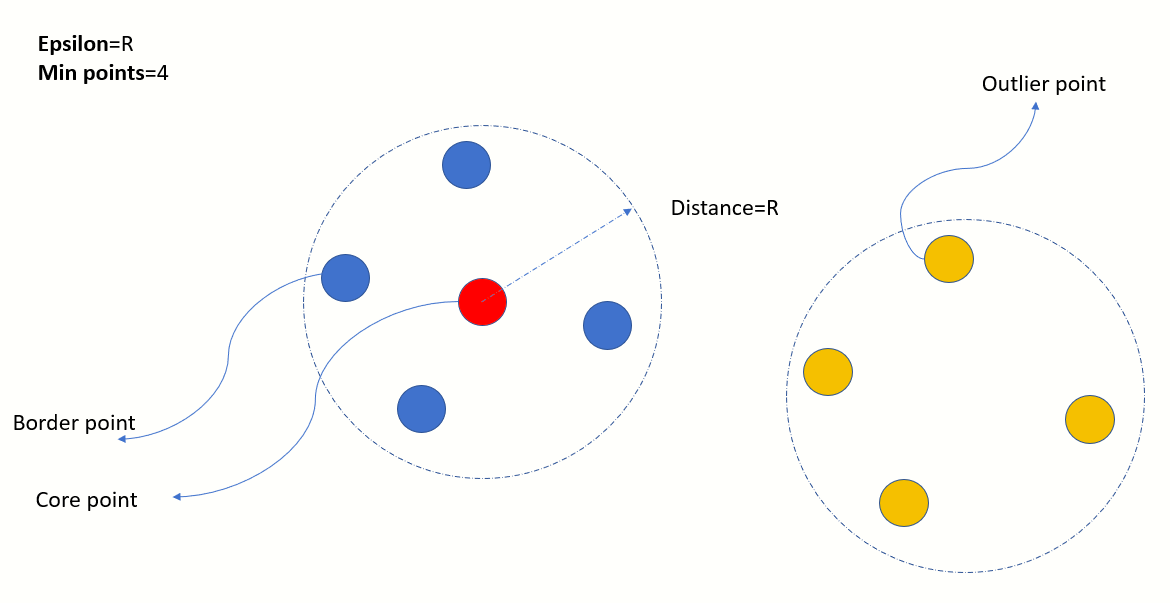
A neighbourhood of a point is defined as the circular region with that point as the centre and a radius of Epsilon. Every point in the dataset is classified into one of the following:

Core point - If there are MinPoints in the neighbourhood
Border point - If this point lies in the neighbourhood of a core point and itself has less than MinPoints in its own neighbourhood
Outlier point - Has less than MinPoints in its own neighbourhood and no other core point in its own neighbourhood

All core points lead to the formation of a cluster. If two clusters have 2 or more core points in their mutual neighbourhood then that cluster is merged. After this iterative process we are left with clusters and outlier points

In-depth understanding of DBSCAN

For a full understanding of the DBSCAN algorithm I recommend this video from Coursera

Very simple code snippet to demonstrate DBSCAN

In the following snippet we demonstrate a very simple usage of the Scikit's DBSCAN algorithm implementation. The input to the algorithm is an array of vectors (2d points in this case) and the output is a 1-dimensional array of integers which denote the cluster label for each and very input vector. E.g. [0, 0, 1, 1, -1, 0, 0, 2, 2, 2, 0, -1, 0] implies there are 3 clusters identified with the labels 0, 1, 2 and 2 outliers denoted by -1.

Sample python code using Scikit learn

import matplotlib.pyplot as plt
from sklearn.cluster import DBSCAN
        
def create_data():
    src_points=[[10,10],[20,20],[30,30]]
        
    src_points.append([9.0,9.0])
    src_points.append([9.5,9.0])
    src_points.append([9.0,9.5])
    src_points.append([9.1,9.8])
        
    src_points.append([20.0,20.0])
    src_points.append([20.1,20.9])
    src_points.append([20.5,20.5])
    src_points.append([20.2,20.8])
        
    src_points.append([30.0,30.0])
    src_points.append([30.5,30.0])
    src_points.append([30.0,30.5])
    src_points.append([30.2,30.8])
    src_points.append([30.8,30.2])
        
    #add some outliers
    src_points.append([1,1])
    src_points.append([40,40])
    return src_points
        
def find_dbscan_clusters(data):
    data_points=data
    epsilon=1
    min_samples=2
    db=DBSCAN(eps=epsilon, min_samples=min_samples)
    db.fit(data_points)
    return db.labels_
        
def display_clusters(data,cluster_and_noise_labels:[]):
    cluster_labels= set(filter(lambda  l: l!=-1, cluster_and_noise_labels))
    count_of_outliers=len(list(filter(lambda  l: l==-1, cluster_and_noise_labels)))
    print("Total clusters produced:%d" % (len(cluster_labels)))
    print("Total outliers produced:%d" % (count_of_outliers))
        
    data_points=data
        
    #Plot the original data points
    x=list(map(lambda p: p[0],data_points))
    y=list(map(lambda p: p[1],data_points))
        
    fig, axs = plt.subplots(2)
    plt.subplots_adjust(hspace=0.5)
    fig.suptitle('Demo of DBSCAN')
    axs[0].scatter(x, y,s=5,c='orange')
    axs[0].set_title("Original points")
        
    #Plot the clusters and outliers
    axs[1].set_title("Clusters ")
    colors=["red","orange", "blue"]
    tuples_of_data_points_class_labels=list(zip(x,y,cluster_and_noise_labels))
        
    unique_labels=set(cluster_and_noise_labels)
    for label in unique_labels:
        noisy_points=list(filter(lambda t: t[2] == label,tuples_of_data_points_class_labels))
        point_x = list(map(lambda  p:p[0],noisy_points))
        point_y = list(map(lambda  p:p[1],noisy_points))
        if (label == -1):
            axs[1].scatter(point_x, point_y, marker='x', label="Outlier")
        else:
            legend_label="Cluster %d" % (label)
            axs[1].scatter(point_x, point_y, marker='o', label=legend_label, c=colors[label])
    axs[1].legend(loc="upper left")
    plt.show()
        
toy_data=create_data()
cluster_and_noise_labels=find_dbscan_clusters(toy_data)
display_clusters(toy_data,cluster_and_noise_labels)

What happens when the dimensions of a feature have different units of measurements?

Consider the clustering scenario on a toy dataset where the dimensions are Height and Weight of students. I have used the Height-Weight chart from NHS United Kingdom as a reference.

As seen from the above plot, in this toy dataset the points are scattered into 2 distinct clusters

Challenge - How to determine epsilon when with 2 different units of measurements on X and Y axis?

The parameter Epsilon can be imagined as the permitted variation while defining a cluster boundary. In this example we could use a permitted variation of 1 Kg along the Weight axis and 10 cm along the Height axis. But, before we compute Epsilon, we will need to re-scale both the axis to the same measurement system. Let us attempt to normalize the data using the MinMaxScaler class

Accompanying Python code

import matplotlib.pyplot as plt
from sklearn.cluster import DBSCAN
from sklearn.preprocessing import MinMaxScaler
import math

def create_height_weight_data():
    src_points=[]
    src_points.append([160.0,60.0])
    src_points.append([160.0,61.0])
    src_points.append([161.0,59.0])
    src_points.append([159.0,61.0])

    src_points.append([180.0,80.0])
    src_points.append([179.0,81.0])
    src_points.append([179.0,82.0])
    src_points.append([180.0,82.0])

    #add some outliers
    src_points.append([170.0,42.0])
    return src_points

def find_dbscan_clusters(data_points):
    scaler = MinMaxScaler()
    scaler.fit(data_points)
    max_weight_variation=1  #1 Kg
    max_height_variation=10 #10 cm

    normalized_zero_zero=scaler.transform([[0,0]])
    normalized_thresholds=scaler.transform([[max_height_variation,max_weight_variation]])

    normalized_height_epsilon=normalized_thresholds[0][0]-normalized_zero_zero[0][0]
    normalized_weight_epsilon=normalized_thresholds[0][1]-normalized_zero_zero[0][1]
    
    epsilon=math.sqrt(normalized_height_epsilon**2 + normalized_weight_epsilon**2)
    min_samples=2
    normalized_data_points=scaler.transform(data_points)

    db=DBSCAN(eps=epsilon, min_samples=min_samples)
    db.fit(normalized_data_points)
    return db.labels_,normalized_data_points

def display(data_points:[],normalized_ht_wt_data:[],cluster_and_noise_labels:[]):
    #Plot the original data points
    x_axis_limits=[100,200]
    y_axis_limits=[20,120]

    x=list(map(lambda p: p[0],data_points))
    y=list(map(lambda p: p[1],data_points))

    fig, axs = plt.subplots(2)
    plt.subplots_adjust(hspace=0.5)
    #fig.suptitle('Demo of DBSCAN')
    axs[0].scatter(x, y,s=10,c='blue')
    axs[0].set_title("Height Weight")
    axs[0].set_xlim(x_axis_limits)
    axs[0].set_ylim(y_axis_limits)
    axs[0].set_xlabel("Height")
    axs[0].set_ylabel("Weight")

    #Plot the clusters
    axs[1].set_title("Clusters ")
    colors=["red","orange", "blue"]
    tuples_of_data_points_class_labels=list(zip(x,y,cluster_and_noise_labels))

    unique_labels=set(cluster_and_noise_labels)
    for label in unique_labels:
        noisy_points=list(filter(lambda t: t[2] == label,tuples_of_data_points_class_labels))
        point_x = list(map(lambda  p:p[0],noisy_points))
        point_y = list(map(lambda  p:p[1],noisy_points))
        if (label == -1):
            axs[1].scatter(point_x, point_y, marker='x', label="Outlier")
        else:
            legend_label="Cluster %d" % (label)
            axs[1].scatter(point_x, point_y, marker='o', label=legend_label, c=colors[label])
    axs[1].legend(loc="upper left")
    axs[1].set_xlim(x_axis_limits)
    axs[1].set_ylim(y_axis_limits)
    axs[1].set_xlabel("Height")
    axs[1].set_ylabel("Weight")

    plt.show()
    pass

ht_wt_data=create_height_weight_data()
cluster_and_noise_labels, normalized_ht_wt_data=find_dbscan_clusters(ht_wt_data)
display(ht_wt_data,normalized_ht_wt_data,cluster_and_noise_labels)

Conclusion and feedback

DBSCAN is a robust algorithm whose outcome depends heavily on the parameters Epsilon and MinPoints. The choice of Epsilon is influenced by the domain. E.g., Creating clusters from the coordinates of stars in the Milky Way and finding clusters of bacterial growth on a Microscope slide would need different values of Epsilon. If the data is naturally spatial, e.g., Latitude, Longitude then determining Epsilon is not so complex. However, when the dimensions have different units of measurements then normalization provides a way forward.

I look forward to hearing your feedback. How would you deal with such a problem?